Fast Algorithm for Monitoring Data Streams by Using Hidden Markov Models

1.1 Problem definition

Increasing the speed of computing HMM likelihoods remains a major goal for the speech recognition community. This is because most of the total processing time (30–70%) in speech recognition is used to compute the likelihoods of continuous density HMMs. Replacing continuous density HMMs by discrete HMMs is a useful approach to reducing the computation cost [1]. Unfortunately, the central processing unit cost still remains excessive, especially for large datasets, since all possible likelihoods are computed.

Recently, the focus of data engineering has shifted toward data stream applications [2]. These applications handle continuous streams of input from external sources such as a sensor. Therefore, we address the following problem in this article:

Problem Given an HMM set and a subsequence of data stream X = (x₁, x₂, ..., x_n), where xn is the most recent value, identify the model whose state sequences have the highest likelihood, estimated with respect to X, among the set of HMMs by monitoring the incoming data stream.

Key examples of this problem are traffic monitoring [3], [4] and anomaly detection [5], [6].

1.2 New contribution

We have previously proposed a method called SPIRAL that offers fast likelihood searches for static sequences [7]. In this article^*, it is extended to data streams; this extended approach, called SPIRAL-Stream, finds the best model for data streams [8]. To reduce the search cost, we (1) reduce the number of states by clustering multiple states into clusters to compute the approximate likelihood, (2) compute the approximate likelihood with several levels of granularity, and (3) prune low-likelihood state sequences that will not yield the best model. SPIRAL-Stream has the following attractive characteristics based on the above ideas:

To achieve high performance and find the exact answer, SPIRAL-Stream first prunes many models by using approximate likelihoods at a low computation cost. The exact likelihood computations are performed only if absolutely necessary, which yields a drastic reduction in the total search cost.

The remainder of this article is organized as follows. Section 2 overviews some background of HMMs. Section 3 introduces SPIRAL-Stream and shows how it identifies the best model for data streams. Section 4 presents the results of our experiments. Section 5 is a brief conclusion.

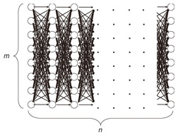
2.1 Definitions

Unlike the regular Markov model, in which each state corresponds to an observable event, an HMM is used when there is a set of unobserved, thus hidden, states and the observation is a probabilistic function of the state. Let {u_i} (i = 1, ..., m) be a set of states. An HMM is composed of the following probabilities:

- Initial state probability π = {π_i}: The probability of the state being u_i (i = 1, ..., m) at time t.

- State transition probability a = {a_ij}: The probability of the state transiting from state u_i to u_j.

- Symbol probability b(v) = {b(v)}: The probability of symbol v being output from state u_i.

HMMs are classified by the structure of the transition probability. Ergodic HMMs, or fully connected HMMs, have the property that every state can be reached from every other state. Another type of HMM is the left-right HMM; its state transitions have the property that, as time increases, the state number increases or stays the same.

2.2 Viterbi algorithm

The well-known Viterbi algorithm is a dynamic programming algorithm for HMMs that identifies the most-likely state sequence with the maximum probability and estimates its likelihood given an observed sequence. The state sequence, which gives the likelihood, is called the Viterbi path. For a given model, the likelihood P of X is computed as follows: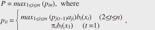

where m is the length of the sequence, n is the number of states, and p_it is the maximum probability of state u_i at time t. The likelihood is computed on the basis of the trellis structure shown in Fig. 1, where states lie on the vertical axis and sequences are aligned along the horizontal axis. The likelihood is computed using the dynamic programming approach that maximizes the probabilities from previous states (i.e., each state probability is computed using all previous state probabilities, associated transition probabilities, and symbol probabilities).

Fig. 1. Trellis structure.

The Viterbi algorithm generally needs O(nm²) time since it compares m transitions to obtain the maximum probability for every state; that is, it requires O(nm²) in each time tick. The naive approach to monitoring data streams is to perform this procedure each time a sequence value arrives. However, considering the high frequency with which new values will arrive, more efficient algorithms are needed.

3.1 Ideas behind SPIRAL-Stream

Our solution is based on three ideas: likelihood approximation, multiple granularities, and transition pruning. These are outlined below in this subsection and explained in more detail in subsections 3.2–3.4.

(1) Likelihood approximation

In a naive approach to finding the best model among a set of candidate HMMs, the Viterbi algorithm would have to be applied to all the models, but the algorithm’s cost would be too high when it is applied to the entire set of HMMs. Therefore, we introduce approximations to reduce the high cost of the Viterbi algorithm solution. Instead of computing the exact likelihood of a model, we approximate the likelihood; thus, low-likelihood models are efficiently pruned.

The first idea is to reduce the model size. For given m states and granularity g, we create m/g states by merging similar states in the model (Fig. 2(a)), which requires O(nm²/g²) time to obtain the approximate likelihoods instead of the O(nm²) time demanded by the Viterbi algorithm solution. We use a clustering approach to find groups of similar states and then create a compact model that covers the groups. We refer to it as the degenerate model.

Fig. 2. Basic ideas behind SPIRAL.

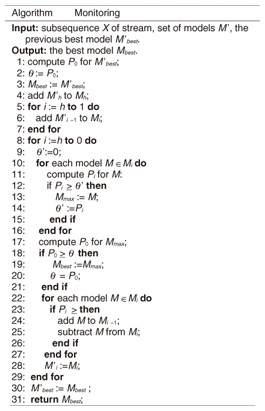
(2) Multiple granularities

Instead of creating degenerate models at just one granularity, we use multiple granularities to optimize the tradeoff between accuracy and comparison speed. As the size of a model increases, its accuracy improves (i.e., the upper bounding likelihood decreases), but the likelihood computation time increases. Therefore, we generate models at granularity levels that form a geometric progression: g = 1,2,4,..., m, where g = 1 gives the exact likelihood while g = m means the coarsest approximation. We then start from the coarsest model and gradually increase the size of the models to prune unlikely models; this improves the accuracy of the approximate likelihood as the search progresses (Fig. 2(b)).

(3) Transition pruning

Although our approximation technique can discard unlikely models, we still rely on exact likelihood computation to guarantee the correctness of the search results. Here, we focus on reducing the cost of this computation.

The Viterbi path shows the state sequence from which the likelihood is computed. Even though the Viterbi algorithm does not compute the complete set of paths, the trellis structure includes an exponential number of paths. Clearly, exhaustive exploration of all paths is not computationally feasible, especially for a large number of states. Therefore, we ask the question: Which paths in the structure are not promising to explore? This can be answered by using a threshold (say θ).

Our search algorithm that identifies the best model maintains the candidate (i.e., best-so-far) likelihood before reporting the final likelihood. Here, we use θ as the best-so-far highest likelihood. θ is updated, i.e., increased, when a more promising model is found during search processing. Note that we assume that no two models have exactly the same likelihoods.

We exclude the unlikely paths in the trellis structure by using θ, since θ never decreases during search processing. If the upper bounding likelihood of paths that pass through a state is less than θ, that state cannot be contained in the Viterbi path, and we can safely discard these paths, as shown in Fig. 2(c).

3.2 Likelihood approximation

Our first idea involves clustering states of the original models and computing upper bounding likelihoods to achieve reliable model pruning.

3.2.1 State clustering

We reduce the size of the trellis structure by merging similar states in order to compute likelihoods at low computation cost. To achieve this, we use a clustering approach. Given granularity g, we try to find m/g clusters from among the m original states. First, we describe how to compute the probabilities of a new degenerate model; then, we describe our clustering method.

We merge all the states in a cluster and create a new state. For the new state, we choose the highest probability among the probabilities of the states to compute the upper bounding likelihood (described in subsection 3.2.2). We obtain the probabilities of new state U_c by merging all the states in cluster C as follows.

We use the following vector of features F_i to cluster state u_i.

where s is the number of symbols. We choose this vector to reduce the approximation error. The highest probabilities are the probabilities of a new state. Therefore, the greater the difference in probabilities possessed by the two states, the greater the difference in the vectors becomes. Thus, a good clustering arrangement can be found by using this vector.

In our experiments, we used the well-known k-means method to cluster states where the Euclidean distance is used as a distance measure. However, we could exploit BIRCH [9] instead of the k-means method, the L1 distance as a distance measure, or singular value decomposition to reduce the dimensionality of the vector of features. The clustering method is completely independent of SPIRAL-Stream and is beyond the scope of this article.

3.2.2 Upper bounding likelihood

We compute approximate likelihood 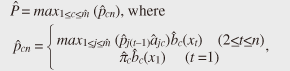from degenerate models that have (=m/g)states. Given a degenerate model, we compute its approximate likelihood as follows:

where is the maximum probability of states.

Theorem 1 For any HMM model, P ≤ holds.

Proof Omitted owing to space limitations.

Theorem 1 provides SPIRAL-Stream with the property of finding the exact answer [8].

3.3 Multiple granularities

The algorithm presented in subsection 3.2 uses a single level of granularity to compute the approximate likelihood of a degenerate model. However, we can also exploit multiple granularities. Here, we describe the gradual refinement of the likelihood approximation with multiple granularities. In this subsection, we first describe the definition of data streams and then our approach for data streams.

In data stream processing, the time interval of interest is generally called the window and there are three temporal spans for which the values of data streams need to be calculated [10]:

This article focuses on the sliding window model because it is used most often and is the most general model. We consider a data stream as a time-ordered series of tuples (time point, value). Each stream has a new value available at each time interval, e.g., every second. We assume that the most recent sample is always taken at time n. Hence, a streaming sequence takes the form (..., x₁, x₂, ..., x_n). Likelihoods are computed only with n values from the streaming sequence, so we are only interested in subsequences of the streaming sequence from x₁ to x_n.

For data streams, we use h + 1 distinct granularities that form a geometric progression g_i = 2ⁱ (i = 0,1,2, ..., h). Therefore, we generate trellis structures of models that have states. Here, g_h represents the smallest (coarsest) model while g₀ corresponds to the original model, which gives the exact likelihood. In the previous our study for static sequences [7], we first compute the coarsest structure for all models. We then obtain the candidate and the exact likelihood θ. If a model has an approximate likelihood smaller than θ, that model is pruned with no further computation. Otherwise, we compute a finer-grained structure for that model and check whether the approximate likelihood is smaller than θ. We iterate this check until we reach g₀.

For data streams, model granularity can be more efficiently decided by referring to the immediately prior granularity for data streams. It is reasonable to expect that the likelihood of the model examined for the subsequence will change little and that we can prune the models efficiently by continuing to use the prior granularities. That is, in the present time tick, the initial granularity is set relative to the finest granularity in the previous time tick at which the model likelihood was computed. If model pruning was conducted at the coarsest granularity, we use this granularity in the next time tick; otherwise, we use the granularity level that is one step down (coarser) as the initial granularity. If the model is not pruned at the initial granularity, the approximate likelihood of a finer-grained structure is computed to check for model pruning against the given θ.

Example If the original HMM has 16 states and the model was pruned with the 1-state model (granularity g₄, coarsest), we choose to use the 1-state model (granularity g₄) as the initial model in the next time tick; if the model is pruned using the approximate likelihood of 16 states (granularity g₀), we select the 8-state model (granularity g₁) as the initial model.

3.4 Transition pruning

We introduce an algorithm for computing likelihoods efficiently on the basis of the following theorem:

Lemma 1 Likelihoods of a state sequence are monotonically nonincreasing with respect to X in the trellis structure.

Proof Omitted owing to space limitations.

We exploit the above lemma in pruning paths in the trellis structure. We introduce e_it, which indicates a conservative estimate of likelihood p_it, to prune unlikely paths as follows: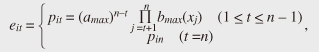

where a_max and b_max(v) are the maximum values of the state transition probability and symbol probability, respectively:

a_max=max_i,j(a_ij), b_max(v)=max_ib_i(v),(i=1,...,m; j=1,..., m).

The estimate is exactly the same as the maximum probability of u_i when t = n. Estimate e_it, the product of the series of the maximum values of the state transition probability and symbol probability, has the upper bounding property assuming that the Viterbi path passes through u_i at time t.

Theorem 2 For paths that pass through state u_i(i = 1, ..., m) at time t(1 ≤ t ≤ n), pjn ≤ eit holds for any state u_j(j = 1, ..., m) at time n.

Proof Omitted owing to space limitations.

This property enables SPIRAL-Stream to search for models exactly.

In search processing, if e_it gives a value smaller than θ (i.e., the best-so-far highest likelihood in the search processing for the best model), state u_i at time t for the model cannot be contained in the Viterbi path. Accordingly, unlikely paths can be pruned with safety.

3.5 Search algorithm

Our approach to data stream processing is shown in Fig. 3. Here, M_i represents the set of models for which we compute the likelihood of granularity g_i, and M'_i represents the set of models computed with the finest granularity in the previous time tick, g_i. SPIRAL-Stream first computes the initial value of θ on the basis of the best model at the last time; it then sets the initial granularity. If a model is pruned at the coarsest granularity at the last time tick, SPIRAL-Stream uses this granularity as the initial granularity. Therefore, we add M'_h to M_h in this algorithm. The one-step-lower granularity is used as the initial granularity if the model was not pruned at the coarsest granularity; this procedure is expressed by “add M'_i-1 to M'_i”.

Fig. 3. Search algorithm.

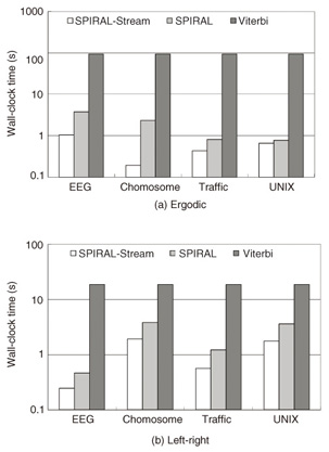
3.6 Theoretical analysis

In this subsection, we provide a theoretical analysis that shows the accuracy and complexity of SPIRAL-Stream.

Theorem 2 SPIRAL-Stream guarantees the exact answer when identifying the model whose state sequence has the highest likelihood.

Proof Let M_best be the best model in the dataset and θ_max be the exact likelihood of M_best (i.e., θ_max is the highest likelihood). Moreover, let P_i be the likelihood of model M for granularity g_i and θ be the best-so-far (highest) likelihood in the search process. From Theorems 1 and 2, we obtain P₀ ≤ P_i, for any granularity g_i, for any M. For M_best, θ_max ≤ P_i holds. In the search process, since θ is monotonically nondecreasing and θ_max ≥ θ, the approximate likelihood of M_best is never lower than θ, where θ is monotonically nondecreasing. The algorithm discards M if (and only if) θ > P_i. Therefore, the best model M_best cannot be pruned erroneously during the search process.

4.1 Experimental data and environment

We used four standard datasets in the experiments.

The models were trained by the Baum-Welch algorithm [11]. In our experiments, the sequence length was 256 and possible transitions of a left-right model were restricted to only two states, which is typical in many applications.

We evaluated the search performance mainly by measuring the duration using a wall clock. All experiments were conducted on a Linux quad 3.33 GHz Intel Xeon server with 32 GB of main memory. We implemented our algorithms using the GCC compiler. Each result reported here is the average of 100 trials.

4.2 Results of data stream monitoring

We conducted several experiments to test the effectiveness of our approach for monitoring data streams.

4.2.1 Search cost

In Figs. 4(a) and (b), SPIRAL-Stream is compared with Viterbi and with the state-of-the-art approach for data sequences, SPIRAL, which finds the best model for static sequences, in terms of the wall-clock time for various datasets where the number of states and number of models are 100 and 10,000, respectively. As expected, SPIRAL-Stream outperformed the other two algorithms: In particular, SPIRAL-Stream could find the best model up to 490 times faster than the Viterbi algorithm.

Fig. 4. Wall-clock time for monitoring data stream.

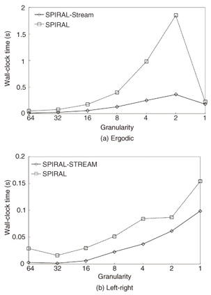
4.2.2 Effectiveness of the data stream algorithm

Our stream algorithm (SPIRAL-Stream) automatically changes the granularity and effectively sets the initial candidate to find the best model. To determine the effectiveness of these ideas, we plotted the time at each granularity for SPIRAL-Stream and SPIRAL. The results of time versus granularity in the model search cost for 10,000 models for EEG, where each model has 100 states, are shown in Figs. 5(a) and (b).

Fig. 5. Breakdown of search cost.

SPIRAL-Stream required less computation time at each granularity. Instead of using g_h (the coarsest) as the initial granularity for all models, this algorithm sets the initial granularity with the finest granularity at the prior time tick, which ensures that the algorithm reduces the number of models at each granularity. Furthermore, the stream algorithm sets the best model at the prior time tick as the initial candidate, which is expected to remain the answer. As a result, it can find the best model for data streams much more efficiently.