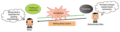
Regular Articles

Vol. 15, No. 3, pp. 33–47, Mar. 2017. https://doi.org/10.53829/ntr201703ra1

An Interpersonal Sentiment Quantification Method Applied to Work Relationship Prediction

Miyuki Imada, Kei Hirose, Manabu Yoshida,
Sun Yong Kim, Naoya Toyozumi, Guillaume Lopez,
and Yutaka Kano

Abstract

For a business to be successful, it is important for people in the business to consider how other people feel, that is, to consider interpersonal sentiment. Our research goal is to quantitatively predict the strength of interpersonal sentiment by analyzing a small amount of data on office employees, for example, their gender or age group, and data on events such as giving positive feedback on work done and sexual or power harassment without directly asking someone about their change in sentiment. In this article, we propose an interpersonal-sentiment-changing model for this quantification and propose two new analysis methods for developing prediction formulas. These methods can be used even if 90% of data is missing and in environments in which it is difficult to gather data in a comparatively short time. We also implement two visualization systems to predict how interpersonal sentiment changes for each event based on actual office data.

Keywords: interpersonal-sentiment prediction, sparse regression, factor regression, visualization, missing data, personal relationships in offices

1. Introduction

For a business to be successful, it is important for the people involved to consider a mental model for work relationships. Let us consider one office scenario (Fig. 1). There are two people, a boss (Boss) and a subordinate (Mike). The relationship between the two is normally positive. One day, Boss yelled at Mike in front of everyone. Boss believed that being strict is important for guiding subordinates and gains a sense of superiority by acting in this manner toward Mike. However, Mike feels he is being harassed and feels contempt toward Boss. Thus, Boss and Mike have opposite interpersonal sentiments, and this affects the other people in the office. These unmatched emotions can negatively affect relationships if nothing is done. Therefore, it is important to make Boss aware that Mike feels contempt toward him in these instances. In other words, Mike’s interpersonal sentiment for Boss can be predicted, and a function is needed that conveys Mike’s sentiments to Boss.

Fig. 1. One office scenario.

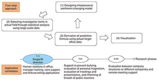
In this article, we describe a way to predict the strength of interpersonal sentiment quantitatively. We statistically predict the strength of interpersonal sentiment by using as little data as possible about office employees, for example, just their gender or age group, without directly asking them whether or not their sentiment has changed. We describe related work and our motivation for this research in section 2. In section 3, we define the interpersonal sentiment discussed in this article. We give an overview of our approach in section 4. In section 5, we explain the proposed interpersonal-sentiment-changing model, and in section 6, we describe how to select investigation items in actual environments through statistical analysis using large-scale data. In section 7, we derive prediction formulas using data from target offices. We evaluate and discuss the estimation accuracy of interpersonal sentiment using these analysis methods. We explain two types of visualization systems for office managers and for office employees in section 8. Finally, we give concluding remarks in section 9.

2. Related work and motivation for this research

In order for businesses that focus on human relationships to succeed, the businesses cannot ignore mental information such as whether people like or dislike something. They also must focus their efforts on a wide range of people (e.g., office employees, students, and teachers) and develop practical interpersonal-sentiment-estimation tools. Interpersonal sentiment has been investigated from two viewpoints, psychological and engineering, and extensive research has been done on the effects of interpersonal sentiment on behavior in personal relationships, for example, parent-child interactions, conflict, negotiation, and leadership. A framework that can account for current findings and guide future research, called the emotions-as-social-information model, has been proposed [1, 2]. Many psychology studies have been conducted from micro- and internal viewpoints and have involved fragmentary trend analysis limited to female students or senior citizens.

There has also been extensive engineering research involving data analysis for automatically recording human behavior using sensors or radio frequency identifiers and web social data [3–5]. Emotion estimation has been investigated using voice and image data analyses [6–8]. Such research goals can be achieved through engineering technology with which people can superficially judge their own emotions by sight. That is, if a person smiles but is inwardly angry, engineering analysis is adequate in only detecting the smile. Thus, many engineering studies have been carried out from macro- and superficial viewpoints. However, the aspect of psychology has not been used in the engineering field.

As mentioned above, we aim to be able to use mental information in applications targeted for humans. However, many psychology studies involved have focused on trend analysis rather than quantification, so psychology research results are difficult to use in applications involving the controlling of human relationships in the workplace. There is currently a wide gap between psychology research and engineering research. We have combined psychology with engineering using statistics, and we use these statistics for sentiment quantification.

3. Interpersonal sentiment

In this article, we describe interpersonal sentiment as the way another person/other people feel. Interpersonal sentiment changes depending on events, and the sentiment has two main aspects, negative and positive. In psychology, interpersonal sentiment consists of several factors [9–13]. We focus on three such factors: like-dislike, respect-contempt, and relief-fear because they greatly concern office managers with regard to their subordinates.

4. Approach for predicting strength of interpersonal sentiment

We applied a four-step approach (explained below) and used the application candidates indicated in Fig. 2. With these candidates, we first clarify the interpersonal sentiment of one-to-one (1:1) relations in single and bi-directions. The application candidates are human relations in offices (target for this article), manager training, care support, and fortune-telling. The next phase involves clarification of interpersonal sentiment in one-to-many relationships (1:n), for example, teacher to students. The application candidates for this type of relationship are prevention of bullying, evaluation of personal magnetism, evaluation of meetings or lectures, and notifying people of breaches in public manners. In the final phase, the approach is expanded to many-to-many relationships (n:m), for example, department-to-department relations. The application candidates are evaluations between company structures or different companies, and remote-meeting support. In this study, we targeted the 1:1 relation of the first phase.

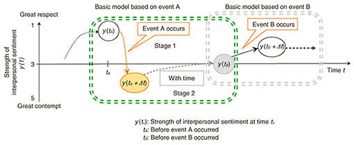
Fig. 2. Approach used in sentiment quantification.

It has not been previously clarified which data are needed to predict the strength of interpersonal sentiment in actual work relationships. We used a statistical method in a top-down approach to identify what types of data are needed for the sentiment prediction. In this approach, we list every conceivable type of data and select from those that are useful (variables) using regression analysis. We follow the following four steps. Steps (1) to (3) are repeated several times to increase the prediction accuracy.

(1) Design of interpersonal-sentiment-changing model

(2) Selection of investigation items in actual offices through statistical analysis using large-scale data

(3) Derivation of prediction formula using actual target office data

(4) Visualization on personal computers (PCs) and smartphones

These steps are described in more detail in the following sections.

5. Design of interpersonal-sentiment-changing model

We developed a model reflecting how our interpersonal sentiments are constructed. A conceptual diagram for changing interpersonal sentiment depending on the event is shown in Fig. 3. The x-axis is the flow of time, and the y-axis is the strength of interpersonal sentiment y. In Fig. 3, we use the interpersonal sentiment factor of respect-contempt as an example. The strength of the sentiment is on a 5-point scale, where 1 represents great respect and 5 represents great contempt, with 3 being neutral.

Fig. 3. Interpersonal-sentiment-changing model.

Let us consider the scenario using Fig. 1. Two people, Boss and Mike, a subordinate, are in an office. They initially respect each other. When event A occurs in which Boss yells at Mike in front of everyone, Mike feels bad due to Boss’ action (stage 1). The strength of interpersonal sentiment regarding respect-contempt before this event y(t_A) decreases from 2 (respect) to 4 (contempt) after the event y(t_A+Δt). However, with time, we usually cool down and return from contempt to a more positive sentiment, 3 (neutral), before the next event (event B) y(t_B) (stage 2). In other words, Mike’s sentiment toward Boss becomes stable over time. After a certain period, event B occurs with similar results to event A. Thus, we argue that stable interpersonal-sentiment results by repeating the combination of stages 1 and 2 several times. Thus, we consider the basic model as consisting of two stages depending on the event.

The prediction goals are as follows.

(1) Small number of variables needed for prediction

We use a regression formula for the interpersonal-sentiment prediction. The regression formula developed using general regression analysis has many variables. Therefore, when we calculate the prediction using the regression formula, we need to prepare the data for these variables. When considering the load for the formula user, we have to reduce the number of variables. Our goal is to have fewer than ten variables.

(2) Estimation accuracy

The estimation accuracy of interpersonal-sentiment strength should be approximately 60–70% with a +/– 0.5 margin of error when using a 5-point Likert scale to rate the three factors mentioned in section 3. We preliminarily interviewed office managers regarding prediction accuracy, and they said that achieving a level of accuracy of approximately 80% was not necessary at first because there has been no quantification of interpersonal sentiment in office environments. They wanted to detect signs of deteriorating situations in the workplace, even if they might be wrong. Therefore, prediction accuracy should be set to higher than 60% on a 5-point Likert scale, although the accuracy rate is 20% stochastically.

6. Selection of investigation items in actual offices through statistical analysis using large-scale data

In this section, we explain the process used to gather and analyze data.

6.1 Acquisition of large-scale data

We gathered calculation data based on our interpersonal-sentiment-changing model illustrated in Fig. 3. We gathered 130 potential explanatory variables for predicting interpersonal sentiment that were referred to in previous psychology and engineering research.

(1) Static variables of responses about oneself

Gender, age group, marital status, with/without children, relatives living together, personality
Occupation, number of employees in company and office, one’s status in the office, one’s value judgment of others

(2) Static variables of responses about others in the office

The others’ statuses in the office, gender, age (older or younger), distance of desk from others (whether two people sit near each other), things in common (e.g., school, hometown, and experiences), how they spend private time, communication tools often used with others (e.g., LINE (social networking app), voice, or email) and duration (e.g., 10 minutes or 1 hour), and how much private information is shared via work email (e.g., if the other is on familiar terms, messages may contain private information such as an invitation to dinner or news about the family.).

(3) Interpersonal sentiment-related variables

We included 83 types of events that may change interpersonal sentiment in the office, for example, power harassment or consoling others regarding work problems.
Respondents’ sentiment when the event occurred and its strength on a 5-point scale. We use Plutchik’s eight primary emotions [14] as the measure of one’s emotions, that is, rage, terror, vigilance, ecstasy, admiration, amazement, grief, and loathing.
Respondents’ condition such as health and deadlines
Initial strength of interpersonal sentiment for each factor with regard to other office staff members
First impressions of others

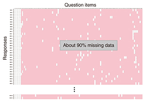
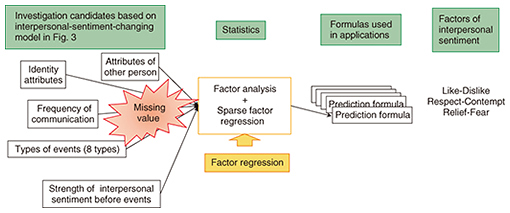
A large amount of data is needed for statistical analysis. We used a web questionnaire as an efficient data-gathering tool for the short term. The web questionnaire was conducted in January 2012. We obtained about 9000 responses.

6.2 Features of web questionnaire data and problem from viewpoint of statistical analysis

(1) Features

Sentiment is subjective; therefore, we have to prepare various choices in order to obtain the truest possible responses. In the first-impression investigation mentioned in section 6.1, we prepared a multiple-choice question asking respondents to choose 10 out of 94 items on what is important regarding first impressions. Each person reacts differently to words, so even if the same impression term was shown, for example, on the appearance of a good-looking man, we provided several words such as cool, cute, good, and smart. In our questionnaires, the respondents all chose the first 6 question items, and the other 4 were random throughout the remaining 88 items.

(2) Problem

As a result, 84 items were not chosen, resulting in a huge amount of missing data, about 90% (shaded region in Fig. 4). Therefore, the method of conventional statistical analysis makes analysis difficult.

Fig. 4. Large amount of missing data.

6.3 Sparse factor regression analysis with large amount of missing data

We used a missing-data algorithm to estimate several of the regression-formula parameters. Regarding our data problem described in section 6.2, we have to determine why the data are missing. Rubin classified the following three types of missing-data mechanisms [15]. The analysis method differs depending on which mechanism is assumed. These mechanisms describe the relationships between measured variables and the probability of missing data.

(1) Missing completely at random (MCAR)

The MCAR mechanism means that data are missing independently of both observed and unobserved data.

(2) Missing at random (MAR)

The MAR mechanism means that when the observed data are given, data are missing independently of unobserved data.

(3) Missing Not at Random (MNAR)

The MNAR mechanism means that missing observations are related to values of unobserved data.

We assume that the missing data (unobserved data) are due to the variable not being chosen from the response. Therefore, we assume the MAR mechanism can be used. We conducted a factor analysis that can be used even if there is a large amount of missing data. Moreover, the factors not derived from factor analysis must be used in regression analysis. We want to minimize the number of useful explanatory variables for interpersonal-sentiment prediction discussed in section 5, even though we listed many candidate variables. Because variables (explanatory variables in regression analysis) may be used as input items in business, for example, in human-relation predictions in an office, having a large number of explanatory variables makes the prediction formula cumbersome and complicated.

The variables chosen from sparse regression modeling are used as the explanatory variables of the interpersonal-sentiment-prediction formula. The number of variables is small, which leads to better privacy protection in service systems because such systems do not need to keep user data that are not necessary for sentiment prediction. As the number of variables decreases, the input load decreases when using the prediction formula.

In this article, we focus on sparse factor regression analysis, and we describe the proposed analysis method based on a large amount of missing data as follows. Let the predictor and responses be x_n and y_n, respectively. In the factor regression model, prediction can be done directly by m latent factors f_n as follows:

where Λ and Θ are factor loadings, and ξ_n and ε_n are error variables. The joint distribution (x_n, y_n) can be expressed as

The above equation can be regarded as a standard factor model:

where and Therefore, we can directly use an estimation algorithm of the factor-analysis model to obtain the solution. An efficient algorithm when a large amount of missing data is involved is detailed in previous papers [16, 17].

6.4 Evaluation results

We proposed the regression formulas for calculating y(t_A+Δt) in Fig. 3 using the method described in section 6.3 (Fig. 5). There are several regression analysis models for obtaining prediction formulas (regression formulas). We used a linear regression model because it is easier to interpret with derived explanatory variables than a non-linear model. Moreover, when we create a graph of discrete values for each variable, the graph shape is not a curve fitting a non-linear model.

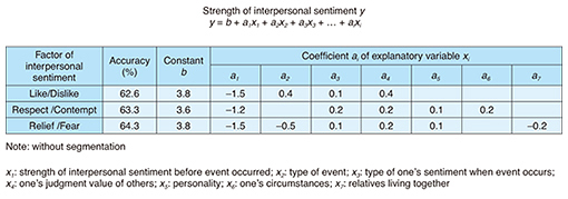
Fig. 5. Overview of factor regression.

The regression formulas and their measured accuracy of interpersonal sentiment are listed in Table 1.

Table 1. Regression formulas and accuracy rates of interpersonal sentiment factors.

The strength of interpersonal sentiment y based on the linear model shown on the y-axis in Fig. 3 is expressed as follows:

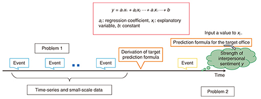
where b is a constant and a_i is a coefficient of explanatory variable x_i (input items of prediction formulas). Three factors of interpersonal sentiment are described in section 3. Our prediction goal was to have ten or fewer variables to reduce the formula user’s load, as explained in section 5. In selecting explanatory variables, we first ensure that the absolute value of a_i is not close to zero since we are using sparse factor regression. Greater absolute values of a_i are useful to estimate y for each factor of interpersonal sentiment. The prediction accuracies listed in Table 1 are the averages of 5-fold cross-validation. We evaluated the prediction accuracy with and without segmentation of all data.

As a result, the prediction accuracy for all three factors was more than 60% without segmentation. We confirmed a prediction accuracy of approximately 70–80% when the data set was divided into several segments using explanatory variables of greater absolute values of a_i, types of events x₂, or initial strength of interpersonal sentiment before an event occurred x₁.

We also found that the approximately 60% accuracy was for all three factors involving only four to six variables (see Table 1, the number of a_i variables). The useful variables were x₁, the initial strength of interpersonal sentiment before an event occurred, x₂, types of events, and x₄, one’s judgment value of others. That is, only up to ten input items at most can be obtained from the prediction formula in which the prediction accuracy is higher than 60%. Conversely, about 120 input candidate items out of the 130 items described in section 6.1 were not useful for predicting interpersonal sentiment.

7. Derivation of prediction formula using actual target office data

Here, we describe how we derived prediction formulas using actual data.

7.1 Problems in gathering data in actual office environment

Statistical analysis is generally necessary for large amounts of data to derive prediction formulas. However, there are two problems with the field data of actual target offices, as shown in Fig. 6 and as follows.

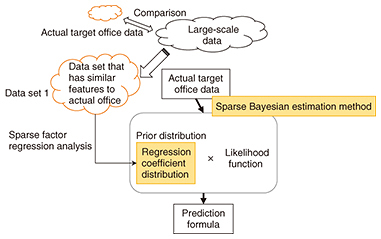
Fig. 6. Process of deriving prediction formula for actual office.

(1) Problem 1

In an actual office, events in which interpersonal sentiments change do not occur frequently. Therefore, a long investigation period such as more than half a year is necessary to acquire an adequate amount of sample data for general statistical analysis.

During a long investigation period, however, personnel changes occur regarding those who are gathering data to develop the prediction formulas. Moreover, office workers who are the subjects of such an investigation bear a heavy burden; thus, the quality of gathered data decreases.

(2) Problem 2

We generally used Bayesian estimation for time-series and small-scale data. The derived prediction formulas using conventional Bayesian estimation consist of many variables. In conventional Bayesian estimation, Markov chain Monte Carlo (MCMC) methods can often be used. MCMC methods find an optimized answer from repeated computations. However, they have heavy computational loads.

In contrast, when we want to minimize the number of variables of a prediction formula, we generally use sparse regression modeling. However, the conventional Bayesian estimation cannot use the standard lasso algorithm (sparse regression modeling).

7.2 Sparse Bayesian estimation method

In this subsection, we describe the method of sparse Bayesian estimation.

7.2.1 Prior distribution of Bayesian estimation using the analysis results of large-scale data

The proposed Bayesian estimation method is depicted in Fig. 7. To overcome problem 1, we use the analysis results of large-scale data through Bayesian estimation. As mentioned in section 7.1, conventional Bayesian estimation is useful to obtain an optimized answer from repeated computations such as with an MCMC method. To obtain an optimized answer with fewer repeated computations, it is important to set appropriate values to the prior distribution. To set the appropriate prior distribution, we propose using the analysis results of sparse factor regression analysis of a large-scale data set gathered from web questionnaires, as described in section 6.1. The data set involves the same kinds of jobs as in actual target offices. Bayesian estimation is generally used as a normal distribution for the prior distribution. Our proposed method uses the regression coefficient distribution obtained from sparse regression analysis for the prior distribution of Bayesian estimation developed using data set 1 in Fig. 7.

Fig. 7. Small-scale data analysis method using large-scale data.

7.2.2 Sparse Bayesian estimation method

To overcome problem 2, we use our method called the sparse Bayesian estimation method to carry out Bayesian estimation and sparse regression.

We focus on the logarithm of posterior distribution on Bayesian estimation used in sequential learning from a few events, which becomes a quadratic function. Bayesian estimation is unified sparse regression that can refine the variables of a prediction formula. We estimate the posterior mode instead of the posterior mean. The estimation of the posterior mode corresponds to the penalized maximum likelihood estimation. The prior distribution is assumed to be a multivariate-normal distribution; therefore, the posterior distribution is also a multivariate-normal distribution, which implies the standard algorithm used in the lasso-type estimation, for example, the coordinate descent algorithm, can be directly used.

The detailed algorithm is described below. The explanatory variables (e.g., gender and age) before an event are denoted as X, and the response variable (degree of connectiveness after the event) is denoted as Y. We conduct linear regression analysis to estimate Y from X, but the number of observations is often small. In this case, the estimator may be unstable. To address this issue, we obtain a stable estimate by using _web, the estimator of parameter θ. Specifically, we use the following posterior distribution:

Note that both likelihood function p(Y|θ, _web, X) and prior distribution p(θ|_web) are multivariate-normal distributions; therefore, the posterior distribution is also a multivariate-normal distribution. The logarithm of likelihood function can then become quadratic.

We consider the sparse estimation of θ via L₁ regularization such as the lasso. Instead of using the negative log-likelihood −log p(Y|θ, _web), we use −log p (Y|θ, _web)−log p(θ|_web). As described above, log p(Y|θ, _web)−log p(θ|_web) takes a quadratic form with respect to θ. When we substitute the above quadratic function with the loss function of the lasso, we can directly use the standard algorithm of the lasso.

7.3 Diary method

We gathered the actual target office data using the diary method that we designed based on the interpersonal-sentiment-changing model shown in Fig. 3. Office employees had to keep a daily diary that includes information such as other staff members’ names, events, and the changes in the strength of their interpersonal sentiments. Approximately 30 of the 130 candidate investigation items were selected through the sparse regression results described in section 6.4, including correction items for the target office.

The 30 investigation items were as follows.

(1) One-time investigation items

Gender, age-group, marital status, with/without children, personality
Types of occupation, one’s status in the office, one’s value judgment of others
Strength of three factors mentioned in section 3 at the initial state for every office staff member

(2) Everyday investigation items

An event that was selected from 83 types of events and Plutchik’s eight emotions mentioned in section 6.1, a 5-point scale on the strength of factors for interpersonal sentiment, and respondents’ condition and situation such as overall health and deadlines.
Staff member’s name involved in the event
Strength of three factors for interpersonal sentiment mentioned in section 3 after the event for all office staff members.

The prediction was y(t_A+Δt) as shown in Fig. 3, and the correct answer values of y(t_A+Δt) are the strength of the three factors after the event.

The data obtained using the diary method to investigate human relations were gathered in four actual offices of an NTT Group company from Oct. 24 to Dec. 15, 2014. The data were input using an HTML (Hypertext Markup Language) interface. Since the interpersonal-sentiment data of office employees were very sensitive, the employees were allowed to answer the questionnaires in the privacy of their homes, as more accurate human-relation data could be gathered.

The basic analysis results of gathering data were as follows.

(1) Office staff (respondent) attributes

Offices (departments): Marketing x 2, Development x 2; total of 4 offices
Males: 17, females: 7
Positions: department managers: 4, department chiefs: 2, staff members: 14, temporary staff members: 4

(2) Number of events that occurred over two months: 167

Positive events: 136
Negative events: 31

(3) Examples of main positive events

Had a positive conversation (mainly marketing offices)
Participated in the same event, drink party, or workshop (all offices)
Helped someone with his/her work (all offices)

(4) Examples of main negative events

Looked down on people (mainly marketing offices)
Refused to take responsibility for problems (mainly development offices)
Exhibited bad manners (mainly marketing offices)

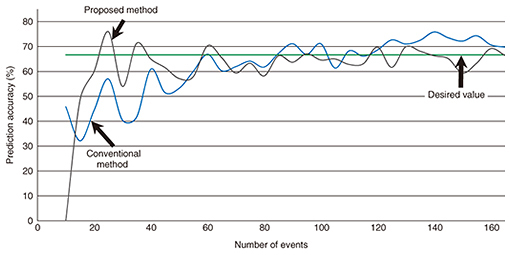
7.4 Evaluation results and discussion

The evaluation results are shown in Fig. 8. The x-axis is the number of events, and the y-axis is the prediction accuracy. We analyzed 167 events that occurred during the two-month investigation period. The factor of interpersonal sentiment was respect-contempt. Data set 1 consisted of about 3100 data samples. The straight green line is the prediction accuracy using sparse factor regression analysis discussed in section 6.3 by using all 167 events. The blue line is the prediction accuracy using the conventional Bayesian estimation method, and the grey line is the prediction accuracy using the proposed sparse Bayesian estimation method. The weight coefficient τ of the initial distribution with the proposed sparse Bayesian estimation method was 1.0. The initial distribution with the conventional Bayesian estimation method was assumed to be uniform (τ = 0).

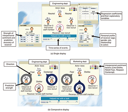
Fig. 8. Prediction accuracy of proposed and conventional methods regarding respect-contempt factor without segmentation.

We checked which of the two methods converged more quickly to the straight line of 67% (desired value) estimation accuracy. Calculations using both methods were started after ten events. The input items were sequentially input using both methods in the order the events occurred. The prediction accuracy of the two methods took an average of five times for two-fold cross-validation of the data of all 167 events.

Both methods began to converge from about 85 events. However, the estimation with the proposed method was more stable than that with the conventional method. That is, the proposed method had less dispersion in estimation accuracy than the conventional method. Therefore, the convergent start point of both methods was almost the same; however, the proposed method became stable faster than the conventional method. There were four useful variables: the initial strength of interpersonal sentiment before an event occurred, types of events, types of occupation, and personality.

Next, we estimated the accuracy enhancement regarding the respect-contempt factor. We focused on the regression coefficient of all data using our diary method. The explanatory variables of a large regression coefficient were gender (= 0.2) and event type (= 0.4). In this article, we have focused on event type, which were segmented into positive and negative events. There were 136 positive events and 31 negative events out of the total 167 events. There were too few negative events for our sparse Bayesian estimation method; therefore, we used the 136 positive events. After data cleansing, we analyzed 111 positive events. The prediction accuracy takes an average of five times for two-fold cross-validation of office data for the 111 positive events. The prediction accuracy was 77%—about 10% higher—by segmentation. Thus, we achieved our prediction goals of obtaining more than 60% prediction accuracy and having ten or fewer variables.

The proposed method converged at about 60 events, and the conventional method converged at about 80 events. That is, the proposed method converged with about one-fourth fewer events than the conventional method. The diary method we used required 30 days to gather the data on 60 events. Thus, we obtained a prediction formula after at least 20 days of learning using the proposed method. This 20-day learning period is sufficient for practical use.

8. Visualization on PCs and smartphones

To our knowledge, no studies have been done on the visualization of human personal relationships from a psychological point of view. We implemented two types of visualization systems. One is for office managers or human resources staff, and the other is for general office staff.

8.1 Visualization system for office managers

We attempted to visualize the change in the prediction of invisible interpersonal sentiment as a tool for managers. We implemented a visualization system as shown in Fig. 9. We prepared two types of visualization displays, a single (Fig. 9(a)) and a comparative visualization screen (Fig. 9(b)). We assumed an actual office scenario in which interpersonal sentiment changes and is easy to visualize in an actual office. In this visualization system, the privacy of responses and an interface for observers were not considered. We will investigate these issues as future work. The comparative visualization display (b) has the same functionality as display (a). The difference is that the interpersonal-sentiment variation in two different departments can be compared for the same events. For example, we can see the difference in interpersonal-sentiment variation between an engineering department and a marketing department.

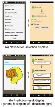
Fig. 9. Visualization for office managers.

The system requirements for visualization are as follows.

Operating system (OS): Mac OS X 10.8.4, HTTP (Hypertext Transfer Protocol) server: Apache 2.2.22, runtime: JDK (Java Development Kit) 7.0_45, browser: Firefox 25, processor: 1.3-GHz dual core Intel Core i5, memory: 4-GB 1600-MHz LPDDR3, storage: 256 GB.

8.2 Visualization system for office staff

In this section, we describe the system to visualize how an office staff member is feeling. The visualization target is the sentiment of a person, so it is very sensitive. It is necessary to carefully investigate changing interpersonal sentiments, depending on who observes the human relations that are visualized. It may be necessary in some cases, for example, when the information made visible is viewed by individual office workers in the workplace, to add minor falsifications of the true predicted values tuned to improve human relations, or to refrain from showing direct information about the people involved in order to protect privacy. To prevent information displayed from being seen by others in the workplace, we implemented the system on smartphones; therefore, users can input data in a private space.

The following components are involved in the visualization process.

First, the gender, age, and position of the person we want to visualize in the organization have to be set. To simplify the relationship information, we decided to allow only the following two types of individuals to be set:

(1) One who provoked an event

(2) One who is affected by having witnessed the event

The prediction of the sentiments between the two set individuals was executed by using the formula mentioned in section 7.2. The data collected from the diary method during in-context experiments were used.

The visualization system was designed as an application for smartphones and implemented on a smartphone. The specifications of the smartphone were as follows.

Smartphone: AQUOS SERIE mini SHV31, central processing unit (CPU): MSM9874AB 2.3-GHz Quad-core, memory: 2 GB, storage: 16 GB, OS: Android 4.4.

In consideration of client-side processing constraints and the high privacy level of manipulated data and results, we implemented the proposed sparse Bayesian estimation method mentioned in section 7.2 using R language, and events or user information files were run or stored on an Apache server.

The server specifications were as follows.

CPU: Intel Core i5-2400 3.1-GHz Quad-core, memory: 8 GB, storage: 128 GB, OS: Windows 10 Pro 64 bit, HTTP: Apache 2.4.17.

The displayed images are shown in Fig. 10. The display combined actual and predicted data; the predicted data were displayed after displaying the actual data collected as the training data set. Specifically, relationships should be expressed through a quiz-style interface such as “Here is the current relationship status; choose the next action and see how the relationship turns out” (Fig. 10(a)). A warning may be displayed when a prediction mismatch occurs (chosen action leads to relationship deterioration). The scenario illustrates the case of monitoring the relationship between colleagues or between full-time and temporary employees. Therefore, the application is suitable for both managerial and subordinate positions. For example, it is possible to input an event such as one that may lead to power harassment, whether you are the actor (the person who provoked the event), the receiver (the person who suffered from the event), or the observer (the person who observed the event). The interface to visualize the prediction of the relationship depending on an event can be a quiz-style interface such as the one mentioned above: “Here is the current relationship status; choose the next action and see how the relationship turns out.” The major functionalities are as follows.

Fig. 10. Visualization for office workers.

Input the identification of the person(s) whose relationship you care about.
Input the related event.
For the user interface, only the top ten most frequent events are displayed first.
For screen size and readability, the event category is selected first; then five to ten concrete events are listed.
Select what action you think would be appropriate next to improve the relationship.
Display the quiz results and prediction accuracy for reference by pressing the relationship-prediction button (Fig. 10(b)).

We used simple sentiments to more easily understand the prediction results, that is, whether the selected next action would be a positive choice. We have conducted demonstrations of this system many times, and it was well received based on the opinions of attendees.

9. Conclusion

The utilization of mental data is important for a business to be successful. In this article, we explained an interpersonal-sentiment-changing model and proposed two analysis methods to quantitatively estimate changes in interpersonal sentiments in an office by using psychological research and statistical data. The first proposed method is a data analysis method that assumes the MAR mechanism, even if about 90% of data is missing. This method is also simultaneously used for sparse regression modeling and factor regression analysis. The second method was a sparse Bayesian estimation method for time-series and small-scale data. For appropriating prior distribution of the method, we used large-scale data that had similar attributes to actual workers in the target offices. The large-scale data were gathered using web questionnaires, and the small-scale data of actual target offices were gathered using a diary method.

With these methods, we achieved a prediction accuracy of more than 60% without segmentation and ten or fewer variables. When we segmented a data set using a variable of a large regression coefficient, the prediction accuracy increased by about 10%.

We finally implemented two types of visualization systems for office managers and for office staff members. Managers can monitor a subordinate’s human relations on a PC, and staff members can monitor relations on smartphones. We demonstrated the visualization systems using actual office data. The demonstrations were well received based on the comments of attendees.

References

[1]	G. A. Van Kleef, “How Emotions Regulate Social Life: The Emotions as Social Information (EASI) Model,” Curr. Dir. Psychol. Sci., Vol. 18, No. 3, pp. 184–188, 2009.
[2]	M. Sinaceur and L. Z. Tiedens, “Get Mad and Get More Than Even: When and Why Anger Expression is Effective in Negotiations,” J. Exp. Soc. Psychol., Vol. 42, pp. 314–322, 2006.
[3]	S. Kumar, F. Morstatter, and H. Liu, “Twitter Data Analytics,” SpringerBriefs in Computer Science (Online), pp. 53–57, 2014.
[4]	facebook, https://www.facebook.com/
[5]	K. Kazama, M. Imada, and K. Kashiwagi, “Characteristics of Information Diffusion in Blogs, in Relation to Information Source Type,” Neurocomputing, Vol. 76, No. 1, pp. 84–92, doi:10.1016/j.neucom.2011.04.036, 2012.
[6]	K. Han, D. Yu, and I. Tashev, “Speech Emotion Recognition Using Deep Neural Network and Extreme Learning Machine,” Interspeech 2014, pp. 223–227, Singapore, Sept. 2014.
[7]	X. Han, R. Elbarougy, M. Akagi, J. Li, T. D. Ngo, and T. D. Bui, “A Study on Perception of Emotional States in Multiple Languages on Valence-Activation Approach,” Proc. of 2015 RISP International Workshop on Nonlinear Circuits, Communications and Signal Processing (NCSP’15), pp. 86–89, Kuala Lumpur, Malaysia, 2015.
[8]	S. Kumano, K. Otsuka, D. Mikami, M. Matsuda, and J. Yamato, “Analyzing Interpersonal Empathy via Collective Impressions,” IEEE Trans. Affective Computing, Vol. 6, No. 4, pp. 324–336, 2015.
[9]	S. J. Breckler, E. C. Wiggins, “Affect Versus Evaluation in the Structure of Attitudes,” J. Exp. Soc. Psychol., Vol. 25, No. 3, pp. 253–271, 1989.
[10]	D. P. French, S. Sutton, S. J. Hennings, J. Mitchell, N. J. Wareham, S. Griffin, W. Hardeman and A. L. Kinmonth, “The Importance of Affective Beliefs and Attitudes in the Theory of Planned Behavior: Predicting Intention to Increase Physical Activity,” J. Appl. Soc. Psychol., Vo. 35, No. 9, pp. 1824–1848, 2005.
[11]	K. Niven, P. Totterdell, and D. Holman, “A Conceptual Classification of Controlled Interpersonal Affect Regulation Strategies,” Emotion, Vol. 9, No. 4, pp. 498–509, doi: 10.1037/a0015962, 2009.
[12]	J. Zaki, W. C. Williams, “Interpersonal Emotion Regulation,” Emotion, Vol. 13, No. 5, pp. 803–810, doi:10.1037/a003383, 2013.
[13]	K. Niven, D. Garcia, I. Löwe, D. Holman, and W. Mansell, “Becoming Popular: Interpersonal Emotion Regulation Predicts Relationship Formation in Real Life Social Networks,” Front Psychol., Vol. 6, doi: 10.3389/fpsyg.2015.01452, published online 2015.
[14]	R. Plutchik, “Emotion: A Psychoevolutionary Synthesis,” Harper & Row, New York, 1980.
[15]	D. B. Rubin, “Inference and Missing Data,” Biometrika, Vol. 63, No. 3, pp. 581–592, 1976.
[16]	K. Hirose, S. Kim, Y. Kano, M. Imada, M. Yoshida, and M. Matsuo, “Full Information Maximum Likelihood Estimation in Factor Analysis with a Lot of Missing Values, arXiv:1312.5458, 2013.
[17]	K. Hirose and M. Imada, “Sparse Factor Regression via Penalized Maximum Likelihood Estimation,” Stat. Papers, online first, 2016. http://link.springer.com/article/10.1007 /s00362-016-0781-8

Trademark notes

Android is a trademark of Google Inc.
Apache is a trademark of the Apache Software Foundation.
AQUOS is a registered trademark of Sharp Corporation.
Intel Core is a trademark of Intel Corporation in the United States and/or other countries.
Java is a registered trademark of Oracle and/or its affiliates.
Mac and OS X are trademarks of Apple Inc., registered in the U.S. and other countries.
Windows is a registered trademark of Microsoft Corporation in the United States and/or other countries.

	Miyuki Imada Senior Researcher, Ubiquitous Service Systems Laboratory, NTT Network Innovation Laboratories. She received an M.E. in education from Yokohama National University in 1990 and a Dr.Eng. in production and systems from Waseda University, Tokyo, in 2005. Since joining NTT Network Service System Laboratories in 1990, she has mainly been involved in researching technology for fault tolerant systems, network security, service emergencies, privacy protection, and pervasive networking. Her current interests include conducting research in the interdisciplinary fields of psychology, engineering, and statistics. Dr. Imada is a member of the Institute of Electronics, Information and Communication Engineers (IEICE).
	Kei Hirose Associate Professor, Kyushu University. He received a Doctor of Functional Mathematics from Kyushu University, Fukuoka, in 2011. His research interests include statistical modeling and machine learning.
	Manabu Yoshida Research Engineer, Ubiquitous Service Systems Laboratory, NTT Network Innovation Laboratories. He received a B.S. in earth sciences and an M.E. in creative science and engineering from Waseda University, Tokyo, in 2008 and 2010. He joined NTT Network Innovation Laboratories in 2010. Since then, his research interests have included ubiquitous computing and affective computing. He was with NTT DOCOMO, where he was involved in service planning, development, and data analytics for marketing from 2013 to 2016. He received the best poster award from the Academy of Human Informatics in 2014. He is a member of IEICE and The Japanese Society for Artificial Intelligence.
	Sun Yong Kim Technical Manager, DOCOMO gacco, Inc. She received her B.E. and M.E. in information science from The University of Tokyo in 2002 and 2004. She was engaged in multivariate analysis and data mining for understanding human behavior and emotions at NTT Network Innovation Laboratories from 2004 to 2013. Since joining DOCOMO gacco, Inc., she has been involved in launching and managing the Japanese MOOC (massive open online course) system named gacco.
	Naoya Toyozumi Graduate Student, Graduate School of Science and Engineering, Aoyama Gakuin University. He received a B.E. in engineering from Aoyama Gakuin University, Tokyo, in 2015. His research interests include signal processing and human machine interfaces.
	Guillaume Lopez Associate Professor, College of Science and Engineering, Aoyama Gakuin University. He received an M.E. in computer engineering from INSA Lyon, and an M.Sc. and Ph.D. in environmental studies from The University of Tokyo in 2000, 2002, and 2005. After working at the Nissan Mobility Research Laboratory for four years, he became Assistant Professor dedicated to the JST CREST Anti-Metabolic syndrome Project (CAMP) in March 2009. He joined Aoyama Gakuin University in 2013, directing the Wearable Environment Information Systems Laboratory. He received the Aoki Award from the Horological Institute of Japan in 2006. His research interests include lifestyle enhancement and healthcare support based on intelligent information systems using wearable sensing technology. His professional memberships include the Academy of Human Informatics, the Institute of Electrical and Electronics Engineers, the Information Processing Society of Japan, the Japan Society of Mechanical Engineers, and the Society of Instrument and Control Engineers.
	Yutaka Kano Professor of Statistics, Graduate School of Engineering Science, Osaka University. He received a D.Eng. in statistics from Osaka University in 1986. He has worked for several schools and universities in Japan including the Department of Mathematics at Tsukuba University and the Graduate School of Human Science and Graduate School of Engineering Science at Osaka University. His interests include statistical science, statistics in social sciences, and statistical education. He was awarded a Research Achievement Prize from the Japan Statistical Society in 2013 and a Lifetime Achievement Prize from the Behaviormetric Society of Japan in 2014. He has also worked as an associate editor for many international academic journals.

↑ TOP