 |
|||||||||||||||||||||||
|
|
|||||||||||||||||||||||
       |
Feature Articles: Efforts to Speed Up Practical Application of Quantum Computers Vol. 21, No. 11, pp. 35–42, Nov. 2023. https://doi.org/10.53829/ntr202311fa4 Quantum Error Mitigation and Its ProgressAbstractCurrent quantum hardware is significantly affected by computation errors. Error reduction is thus required to obtain meaningful results from quantum computers. Quantum error mitigation (QEM) methods, which are a class of hardware-friendly error-reduction methods not relying on the encoding of quantum information, are being actively researched. In this article, I review the major QEM methods. I then introduce the recent progress in QEM technologies proposed by our research group. First, I review the worlds’ first quantum sensing method incorporating QEM. I then review the generalized quantum subspace expansion method, quite a general unified framework of QEM. Keywords: quantum computing, quantum error mitigation, post-processing of measurement results
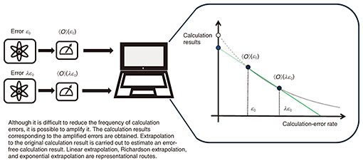
1. Quantum error mitigationA pressing challenge for quantum computers is suppressing the effects of computational errors due to the loss of quantum coherence. Quantum error mitigation (QEM) is a relatively recent concept proposed for mitigating computation errors while keeping the hardware load to a minimum [1]. QEM is often compared with quantum error correction (QEC). In QEC, multiple physical quantum bits (qubits) are used to represent a single logical qubit. This redundancy is used to detect computational errors, and errors are actively corrected on the basis of this information. However, because the number of qubits in quantum hardware is at most several hundred qubits, QEC reduces the effective number of qubits. QEC thus cannot make the best of the computation power of near-term quantum devices. Therefore, QEM was introduced as a set of methods that can reduce computational errors without reducing the effective number of qubits by avoiding the use of redundancy. Progress related to QEM implementation has been remarkable. In a recent paper, IBM claimed the world’s first accomplishment of a practical task with a 127-qubit quantum processor [2]. This breakthrough shows that QEM has an extremely useful role. The exponential-extrapolation error mitigation method I proposed [3] also shows extremely high performance. There are a variety of other QEM methods. In QEM, the correct result of a calculation is generally estimated by post-processing the output from multiple quantum circuits using a classical computer. A conceptual diagram of QEM is shown in Fig. 1(a). QEM cannot fundamentally suppress errors in the quantum state. However, it can mitigate errors in the expectation values of observables. Figure 1(b) illustrates the function of QEM. Because many quantum algorithms that are expected to be implemented in current quantum computers and first-generation fault-tolerant quantum computation use the expectation values of observables, QEM is considered to be highly useful. It should be noted that the cost of QEM is an increase in measurement shots; an exponentially greater number of measurements in accordance with the frequency of computational errors in quantum hardware is required. Intuitively, this is because QEM has the effect of amplifying the expectation values of observables that generally decays exponentially with respect to the number of quantum gates and the gate error rate. The variance of calculation results thus increases exponentially. Mathematical proof related to the exponential increase in the number of measurements have been shown in several papers, including that by our research group [4], using a quantum information-theoretic approach. In the following section, I discuss the major QEM methods: extrapolation [3, 5], quasi-probability (also called probabilistic error cancellation [3, 5]), virtual distillation [6], and subspace expansion [7].
I then describe our research groups’ latest achievements, a quantum sensing method incorporating QEM [8] and quite a general unified framework of QEM called the generalized quantum subspace expansion method [9]. For readers who wish to simply have an overview of QEM, it is sufficient to understand the extrapolation methods. For those who wish to learn more, I encourage you to read the other sections. Referring to the review paper I wrote [1] when needed will provide an in-depth understanding of QEM. 1.1 Extrapolation methodsAs the name suggests, extrapolation methods estimate the ideal error-free calculation result by extrapolating multiple measurement results [3, 5]. They are simple yet powerful methods used in many experiments. An overview of extrapolation methods is shown in Fig. 2. The horizontal axis shows the error rate and the vertical axis shows the result (the expectation value of an observable). Of course, we cannot freely reduce the error rate, but it is relatively easy to increase calculation errors. For example, it is possible to increase the frequency of errors by slowly carrying out gate operations or by carrying out extra gate operations. By extrapolating the original calculation result and calculation results associated with increased error rates, the ideal error-free calculation result is then estimated. When extrapolation methods were first proposed, they used Richardson extrapolation with linear and polynomial functions [5]. Observing that calculation results generally decay exponentially with the frequency of calculation errors, I proposed extrapolation using an exponential function [3]. The exponential extrapolation showed extremely good performance in an actual experiment [2]. However, extrapolation methods cannot guarantee computation accuracy and can be said to be relatively heuristic.
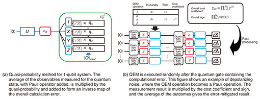
The number of measurements, a cost factor in QEM, can be easily understood with extrapolation methods. Considering linear extrapolation as an example, for calculation error rate ε0, we express the experimentally obtained average value of the observable as ⟨O(ε0)⟩ and that with twice the error rate as ⟨O(2ε0)⟩. From extrapolation, the error-mitigated result can be written as Oest = 2⟨O(ε0)⟩ − ⟨O(2ε0)⟩. When calculating variance, if no correlation is assumed between ⟨O(ε0)⟩ and ⟨O(2ε0)⟩, we obtain Var[Oest] = 4Var[⟨O(ε0)⟩] + Var[⟨O(2ε0)⟩]. This shows that the variance is amplified after applying QEM and that more measurements are needed to obtain the correct calculation result. 1.2 Quasi-probability methodThe quasi-probability method counteracts the effect of gate noise by effectively constructing the inverse of the noise based on the noise model obtained through noise characterization techniques, such as process tomography or gate set tomography [3, 5]. We denote the quantum process corresponding to the noise as Ԑ (it may be easier to think of it as the quantum mechanical version of a transition matrix) and its inverse map as Ԑ−1. While Ԑ−1 can be mathematically constructed, it is not generally a “physical process” and cannot be directly operated on a quantum computer. By constructing Ԑ−1 by a set of operations {Bk}k for QEM that we can execute with fewer calculation errors, we can decompose Ԑ−1 as Ԑ−1 = ∑k qk Bk. Usually, we assume that {Bk}k are single qubit operations. For example, when we consider the depolarizing noise of error probability p to be It is important to implement the inverse map in a quantum circuit with multiple qubits for practical purposes. Consider when a quasi-probability method is applied to the noise Ԑl (l = 1,2,…NG, where NG is the number of gates) of multiple quantum gates. The conceptual diagram is shown in Fig. 3(b). We construct an inverse map for each error:
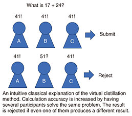
Although a suitable error-characterization method has not been proposed when the quasi-probability was first proposed, I found that gate-set tomography is an efficient error-characterization method for this method [3]. I also discovered a set of operations {Bk}k for QEM that allows for removal of arbitrary computational errors [3]. I have also shown that the quasi-probability method can be applied not only to gate models but also temporally continuous noise models such as those described by the Lindblad master equation 1.3 Virtual distillation methodVirtual distillation executes QEM by preparing multiple copies of a noisy quantum state ρnoisy, executing entanglement measurements between them and post-processing the results using a classical computer. This enables us to simulate the error-suppressed quantum state as if we distill a noiseless quantum [6]. An example of the “classical” counterpart of this method is as follows: we ask several students to solve the same problem, e.g., elementary school students who often get erroneous results for simple arithmetic problems. Only when all the calculation results are the same is the answer submitted; otherwise, the results are discarded (Fig. 4). The more students involved in calculating the result, the higher the percentage of the correct answer. However, the probability of success (i.e., the probability of all students calculating the right answer) decreases exponentially with the number of students.
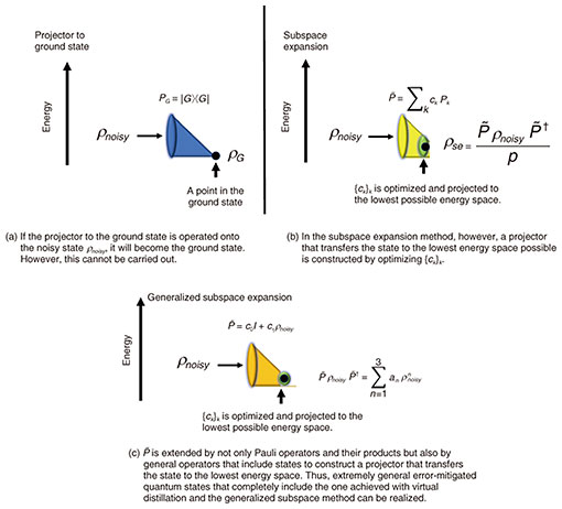
With virtual distillation, we can calculate the expected value of the physical quantity corresponding to the distilled quantum state 1.4 Subspace expansion methodThe subspace expansion method constructs a projector (strictly speaking, this operator does not satisfy the mathematical properties of a projector but is called one here for convenience) [7]. Consider a case in which the actual quantum state immediately before measurement differs from the ideal quantum state because of noise. For example, the variational quantum eigenvalue solver is a method for determining the ground state ρG = |G⟩⟨G| of molecules, etc; however, the actual quantum state may be another quantum state ρnoisy because of errors. If we can construct the projector onto the ground state PG = |G⟩⟨G|, an error-free quantum state can be obtained as
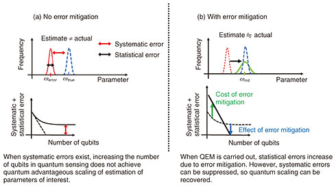
2. NTT’s latest achievements2.1 Application of QEM to quantum sensingNTT has developed the world’s first framework for quantum sensing incorporating QEM. Quantum sensing is an active area of research in the field of quantum information that uses quantum states to efficiently probe fields such as magnetic fields one wishes to measure. This is done by interacting the quantum states with the field followed by the readout. The process is repeated and the results are accumulated to estimate the value of the magnetic field. What is important about quantum sensing is that when quantum entangled states are used as probes, quantum advantageous scaling can be achieved depending on the number of qubits N. However, if the noise fluctuates at each time of measurement, systematic errors occur in the accumulated value and estimated magnetic-field value, and quantum advantages cannot be achieved (Fig. 6(a)). Our research group has shown that even when noise fluctuates each time the quantum device is executed, virtual distillation can act as a “filter” that removes such noise and accurately mitigates systematic errors [8]. We have also shown that quantum advantageous scaling can be restored (Fig. 6(b)).
2.2 Generalized subspace expansion methodOur research group proposed the generalized subspace expansion method, which is quite a general QEM method, which includes subspace expansion and virtual distillation as special cases [9]. I stated above that in subspace expansion, the projection operator References
|
||||||||||||||||||||||