 |
|||||||||||||||||||||||||||||||||||||||||||
|
|
|||||||||||||||||||||||||||||||||||||||||||
       |
Regular Articles Vol. 9, No. 3, pp. 73–82, Mar. 2011. https://doi.org/10.53829/ntr201103ra2 Compressed Sensing Technology for Flexible Wireless SystemAbstractWe are developing a flexible wireless system (FWS) in response to the rapid development of and changes to wireless radio environments. FWS is a unified wireless platform that simultaneously receives various types of wireless signals at distributed remote stations and performs signal processing at the central station by transferring the received radio wave data via the wired access line. As a partial fulfillment of our system, we have applied compressed sensing technology as a radio wave data compression technology for FWS. Compressed sensing is a new framework for solving an ill-posed inverse problem of a sparse signal. Direct translation of compressed sensing in the sense of wireless technology is as follows: radio wave data can be received, transmitted, and reconstructed using sub-Nyquist rate information without aliasing if the original radio wave is sparse. To provide a full understanding of our approach, this article first reviews basic knowledge about compressed sensing and then describes the application scenario of compressed sensing in FWS. 
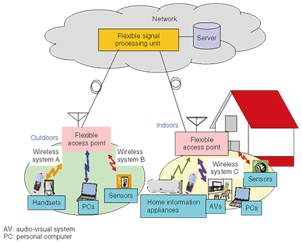
1. IntroductionThe rapid development of and changes to wireless radio environments require a unified platform that can flexibly deal with various wireless radio systems [1]. To satisfy this requirement, we are developing a flexible wireless system (FWS), which is composed of flexible access points and a flexible signal processing unit [2]. The concept of FWS is illustrated in Fig. 1. Multiple wireless signals are simultaneously received by flexible access points, which can receive a wide variety of wireless signals with frequencies ranging from several hundred megahertz to several gigahertz. The received radio wave data is transferred to the flexible signal processing unit through a broadband wired access line. The flexible signal processing unit performs multiple types of signal analysis by software exploiting software defined radio and cognitive radio technologies [3]. If necessary, previously stored data at servers can also be used.
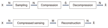
The huge bandwidth necessity for transferring the received radio wave data motivated us to develop a highly flexible and efficient radio wave data compression technology. To accomplish this goal, we applied recently developed compressed sensing technology. Compressed sensing is a new framework for solving an ill-posed inverse problem of a sparse signal [4]. Direct translation of compressed sensing in the sense of wireless technology is as follows: radio wave data can be received, transmitted, and reconstructed using sub-Nyquist rate information without aliasing if the original radio wave is sparse. In relation to FWS, compressed sensing has two advantages. First, it provides universality in wireless signal reception regardless of system types. This provides flexible signal reception because all types of signals can be received by a unified signal reception method. Furthermore, no modifications are necessary even when new wireless systems are introduced. Second, it enables signal reception and reconstruction at a lower rate than the Nyquist rate. This reduces the burden of data transfer between flexible access points and the flexible signal processing unit. The remainder of this article is organized as follows: Section 2 reviews basic knowledge about compressed sensing, section 3 describes our compression method, and section 4 concludes with a brief summary of the main points and a mention of future work. 2. Compressed sensing2.1 Basic conceptA simplified explanation of compressed sensing is as follows: A signal projected linearly onto a lower-dimensional space can be used to reconstruct the original higher-dimensional signal with high probability if the signal is sparse (explained in section 2.2) and the projection matrix satisfies the restricted isometry property (RIP, explained in section 2.4). In a mathematical sense, compressed sensing can be stated as an ill-posed inverse problem. Normally, the solution of an ill-posed inverse problem is not uniquely determined because the number of equations is smaller than the number of variables. However, the solution of an ill-posed inverse problem can be uniquely determined by investigating all possible cases provided that the signal is sparse. Moreover, if an ill-posed inverse problem satisfies RIP and the signal is sparse, the unique solution can be found with a practical degree of complexity. For an intuitive understanding of compressed sensing, consider the following simple ill-posed inverse problem. Find m, n, and k such that m + 3n - 2k = 1 -m – n + k = -1 Normally, the solution is not uniquely determined because the number of equations is smaller than the number of variables. However, if vector [m k n] has only one nonzero element, the unique solution can be obtained by investigating all possible cases, as below. case 1) m≠0, n=k=0 -> m=1 (unique solution) case 2) n≠0, m=k=0 -> impossible case 3) k≠0, m=n=0 -> impossible Although the unique solution is available, this is an NP-hard problem for which all possible cases must be investigated. Consequently, it becomes impractical as the number of dimensions of the signal increases. This impracticality is overcome if the equation vector [1 3 -2; -1 -1 1] satisfies RIP. The core achievement of compressed sensing is that the above NP-hard problem can be cast into an l1-norm minimization problem (explained in section 2.5) if the signal is sparse and RIP is satisfied. L1-norm minimization problems can be solved by linear programming, which is a well established convex optimization method, with practical complexity O(n3) [5], [6]. Considering the above example, the following two statements can be made: First the sparsity of the signal assures the unique solution for compressed sensing. Second, RIP assures a practical degree of complexity for finding the unique solution for compressed sensing. 2.2 Sparse signalA signal is called sparse when it is represented by a small number of nonzero coefficients in any convenient domain. More specifically, N×1 signal X is called S-sparse if X is represented by the multiplication of any N×N transform matrix Ψ and N×1 coefficient vector s, and s has only S nonzero coefficients. The definition of sparsity is not limited to the orthogonal transform domain (i.e., Fourier transform or wavelet transform). If a signal is represented in a non-orthogonal domain, including any user-defined domain, the signal is also called sparse [7]. 2.3 MeasurementFor a given N×1 signal X, measurement is defined as the linear projection of X onto M×1 signal Y. The M×N matrix Φ that casts X onto Y is called the measurement matrix. Matrix description is given by Y=ΦX. If X is represented by N×1 coefficient vector s in the N×N transform domain Ψ , it is expressed as Y=ΦΨs. The number of measurements is the number of rows in the measurement matrix (M), which is also equivalent to the number of dimensions of the output signal. Therefore, the compression rate increases as the number of measurements increases. Numerous studies have been performed to investigate the minimum bound of the necessary number of measurements for a given signal sparsity [8 and references therein]. It has been shown that S•log(N/S) measurements are enough for the reconstruction of an S-sparse signal when measurement matrix Φ consists of random ensembles [9]. 2.4 RIPThe most outstanding achievement of compressed sensing is the fact that RIP casts an NP-hard problem onto an l1-norm minimization method [10], [11]. When an M×N measurement matrix Φ and a N×N transform domain matrix Ψ satisfy the following inequality for all S-sparse vectors, matrix Θ(=ΦΨ) is said to obey RIP of order S with δ. (1-δ)||s||22 ≤||ΦΨs||≤(1+δ)||s||22 where ||s||2=Σi si2 and δ(0 ≤δ <1) is the smallest constant that satisfies the above inequality. An intuitive explanation of RIP is as follows: the Euclidian distance between any two N×1 S-sparse vectors is approximately preserved after the measurement as long as Θ obeys RIP. It has been proven that RIP is satisfied if measurement matrix Φ consists of random ensembles, which yields the following surprising result: any unknown sparse signals can be reconstructed by random measurement [10]. This property provides flexibility for the compression of an unknown signal because signal-independent measurement is possible by the random measurement as long as the signal is sparse. 2.5 ReconstructionReconstruction of the compressed sensing refers to finding N×1 S-sparse vector s from known M×1 measurement output matrix Y, M×N measurement matrix Φ, and N×N transform matrix Ψ when Y=ΦΨs (S<M<<N). Reconstruction of the original signal s can be found via the l1-norm minimization problem, as described below, as long as RIP is satisfied. min||sˆ||1 subject to Y=ΦΨsˆ, sˆ∈RN, if RIP satisfies sˆ=s, where ||sˆ||1=|s1|+|s2|+...|sN| and RN is the set of N×1 vector. The l1-norm minimization problem finds sˆ that minimizes the l1-norm subject to Y=ΦΨsˆ among all possible S-sparse vectors. This seems to be an NP-hard problem, but it can be cast into a convex optimization problem and solved by the linear programming method. Furthermore, if RIP is satisfied, sˆ is identical to the original vector s with high probability [10], [11]. If the measurement matrix consists of random ensembles, flexible reconstruction is possible. In the case that signal X is proved to be more sparsely represented in another basis matrix Ψ’, surprisingly, one does not need to conduct the measurement again since the l1-norm minimization problem can be solved with Y and a new Θ’(=ΦΨ’). This indicates that once the projection has been performed, the reconstruction can be performed with any convenient basis matrix. There are other approaches to the reconstruction of compressed sensing such as an orthogonal matching pursuit algorithm, which uses a greedy iterative algorithm [12]. 2.6 Comparison between conventional compression and compressed sensingThe difference between the conventional compression and compressed sensing is shown in Fig. 2. The conventional sample-then-compress method compresses the signal by the signal-specific compression method, which yields the optimal compression (S dimensions). On the other hand, compressed sensing conducts a signal-independent linear projection of the original signal onto a lower-dimensional space (M-dimensional, S<M<<N), which yields poor compression performance. Therefore, it can be stated that the conventional compression method is superior to compressed sensing for the known signals in terms of compression performance.
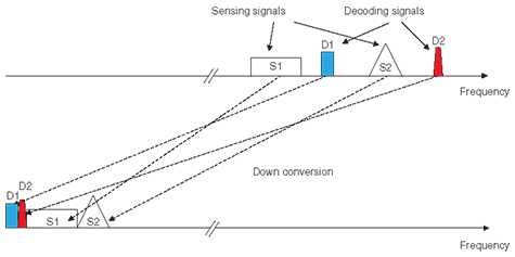
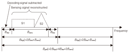
However, compressed sensing has the following advantages compared with the conventional compression method. First, it is suitable for dealing with an unknown sparse signal. Second, it is robust to the introduction of new types of wireless systems. When new types of wireless systems are introduced, receivers (flexible access points in Fig. 1) do not need to be modified because the signal-specific processing burden is moved from the receivers to the server (flexible signal processing unit in Fig. 1). Third, it reduces the burden on receivers. For example, consider a sparse signal of unknown frequency. In the case of the conventional sampling method, receivers must conduct both a fast Fourier transform and a search for nonzero coefficients. On the other hand, in the case of compressed sensing, receivers only need to conduct a linear projection. 3. Application of compressed sensing for FWSThis section describes two radio wave data compression methods that utilize compressed sensing. Both methods try to exploit the flexibility of compressed sensing by utilizing prior information. One method uses a random sparse measurement matrix based on random sampling [13] (or equivalently, random discard from all of the sampled data). The other uses a random dense measurement matrix that conducts a full linear projection of sampled data [14]. 3.1 Combined Nyquist and compressed samplingThe goal of this sampling method is to achieve Nyquist-rate sampling of the known signal (hereinafter called the decoding signal) and compressed-rate sampling of the unknown signal (hereinafter called the sensing signal) in a single analog-to-digital converter. To achieve this goal, the following processes are carried out. At each flexible access point, multiple signals are simultaneously received, filtered, and down-converted to the intermediate frequency (IF) band. In particular, decoding signals are converted to a lower center frequency band than sensing signals, as shown in Fig. 3. Signal down-conversion is done by tunable local oscillators and mixers. All down-converted signals are sampled by our method and transferred to the flexible signal processing unit.
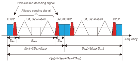
Details of the combined Nyquist and compressed sampling method are as follows. Suppose that L decoding signals and M sensing signals are aligned in the IF band, and the total bandwidths of these signals are represented by Bdec and Bsens, respectively. For the convenience of the explanation, Bgrid and BNyq are defined as (4Bdec+2Bsens) and (2Bdec+Bsens), respectively. The purpose of the above setting is to achieve (1) Nyquist-rate sampling of the decoding signals without aliasing from the sensing signals and (2) compressed-rate sampling of the sensing signals in a single analog-to-digital converter simultaneously. The detailed procedure of our method is as follows. First, Bgrid-rate sampling is conducted. Second, only some of the even (odd) samples are randomly discarded while all of odd (even) samples are preserved. The locations of randomly discarded samples, which are determined by the random sequences generator, can be known to the flexible signal processing unit if the initial seed of the random sequence generator is shared. Hereinafter, all the odd samples and the remaining even samples are called fixed samples and random samples, respectively. They are transferred to the flexible signal processing unit via the wired access line. The mathematical description of our method is as follows. For simplicity, we consider multiple sparse signals in the frequency domain. The IF band signal X=(Ψs) is sparsely represented in the frequency domain. The basis matrix Ψ is an N×N inverse Fourier transform, and s is the N×1 coefficient vector of X in the frequency domain. Note that s has sequential nonzero values in the lower frequency region and randomly sparse nonzero values in the higher frequency region (e.g., s=[1111100100010001]). The K×N projection matrix Φ has the following sparse representation. 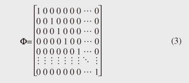 Note that each column indicates a sample point of the signal. Every odd sample is preserved while some of the even samples are randomly discarded. Then, the compressed sensing matrix Θ(=ΦΨ) becomes a K×N matrix consisting of every odd row and randomly selected even rows of the inverse Fourier transform matrix. Projection vector Y is represented by Θs and signal reconstruction becomes the inverse problem of s =Θ-1Y. This inverse problem is solvable as an l1-norm minimization problem because s is sparse and Θ consists of randomly selected rows of the inverse Fourier transform matrix*. Using transferred fixed and random samples from flexible access points, the flexible signal processing unit conducts the decoding and sensing process as follows. First, the decoding signals are decoded using only fixed samples, which is equivalent to BNyq-rate sampling. Note that aliasing of the sensing signals occurs because the sampling rate is insufficient. However, it does not cause interference with the decoding signals. Therefore, the decoding signals can be decoded by using conventional decoding algorithms without aliasing. An example of fixed samples in the frequency domain is shown in Fig. 4. Although the aliasing of the sensing signals occurred owing to the insufficient sampling rate, the decoding signal parts are intact. Consequently, Nyquist-rate decoding performance is achieved for the decoding signals. Second, the decoding signal is subtracted from both the fixed and random samples. Third, the sensing signals are reconstructed using both fixed and random samples, whose decoding signals have been subtracted. The reconstruction is done by solving the l1-norm minimization problem. An example of the reconstructed signal in the frequency domain is shown in Fig. 5. Note that only sensing signals are reconstructed because the decoding signals have been removed. Fourth, the sensing signals are identified in the reconstructed signal by a conventional spectrum sensing algorithm such as energy detection.
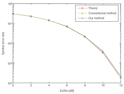
Some experimental results are shown in Figs. 6 and 7. Experiments were performed on 310-MHz-band frequency shift keying (FSK) signals transmitted by radio frequency identification (RFID) tags. The RFID tag bandwidth and the total bandwidths of decoding signals and sensing signals were 0.3, 1.73, and 6.54 MHz, respectively. The channel between the RFID tags and a flexible access point was a non-fading additive white Gaussian noise channel.
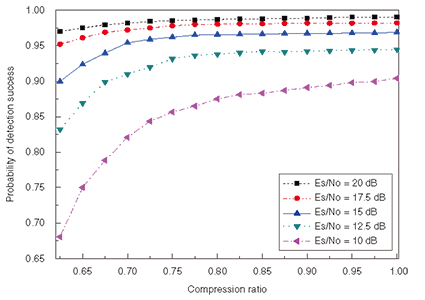
Figure 6 compares the theoretical and experimental symbol error rates for the decoding signal in terms of Es/No (energy per symbol per noise power spectral density). In the experiment using the conventional method, only the down-converted decoding signal was sampled at the Nyquist rate. In the experiment using our method, the decoding signal and the sensing signals were combined in the IF band and sampled by using our method. The performance curve for our method matches those for the theoretical and conventional methods well, which shows that our sampling method guarantees Nyquist-rate decoding performance for the decoding signal. The detection success rate is shown in Fig. 7. All curves show relatively poor performance at a low compression ratio. This is because reconstruction fails if the number of samples is insufficient. However, Pd (detection success rate) increases with the compression ratio. Approximately, 70% of the compression ratio can be achieved when Es/No is higher than 17.5 dB.
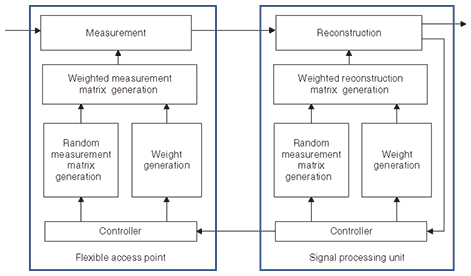
3.2 Compressed sensing with weighted measurement matrixOur goal for the weighted measurement matrix generation is to reduce the required number of measurements by using prior knowledge of the signal. A block diagram of compressed sensing with weighted measurement matrix generation is shown in Fig. 8. The weighted measurement matrix is generated by multiplying the random measurement matrix and weight matrix, where the weight matrix is generated taking into consideration prior knowledge such as the signal’s history. Note that identical weighted and random measurement matrices are generated by both the flexible access points and the signal processing unit for the reconstruction. If the weight needs to be updated, necessary parameters are transmitted from the signal processing unit to the flexible access points.
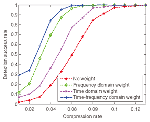
To verify the efficiency of this method, we conducted an experiment using an RFID signal consisting of a periodically transmitted FSK signal. The total bandwidth and the received signal bandwidth were 5 and 0.6 MHz, respectively. The time occupancy rate of the received signal was 0.25. Therefore, the time-frequency domain signal sparsity was 0.03. The time and frequency domain weights were set to 2.0 and 1.5 using the signal reception history. The detection success rates for the conventional method and our method are compared in Fig. 9. The compression rates needed for perfect signal detection were 0.13, 0.12, 0.09, and 0.08, respectively, when the applied weights were no weight, time domain weight, frequency domain weight, and time-frequency domain weight. These results confirm that enhanced compression is achieved by our method.
4. ConclusionTo satisfy the requirement for a unified wireless platform, we are developing a flexible wireless system. As a partial fulfillment of such as system, this article described a highly efficient radio wave data compression method based on currently developed compressed sensing technology. It also described two radio wave data compression methods utilizing compressed sensing technology. Experiments results verified that a compression rate that is slightly higher than the Nyquist rate of the original sparse signal can be achieved. Our future research will include developing further enhanced data compression methods in terms of realtime operation and practical processing burden using compressed sensing technology. References
|
||||||||||||||||||||||||||||||||||||||||||